Agile

Agile is a microwave/RF harmonic balance simulator. It can analyze linear as well as steady-state non-linear circuits and networks. Beyond analysis there are features for optimization and statistical analysis and design.

See this wiki page on harmonic balance if you are not familiar with it — but its a lot simpler conceptually than it appears there, basically harmonic balance assigns a complex-valued (magnitude and phase) voltage at each node for each frequency (harmonic) in the simulation. Given these voltages the resultant currents (at each harmonic) from the linear and non-linear side is computed to determine an error value (some form of difference between the linear and non-linear sides). The voltages are then adjusted until the currents agree, that is the balance. Of course there may be multiple, or no, solutions; and solutions may exist but not be found.

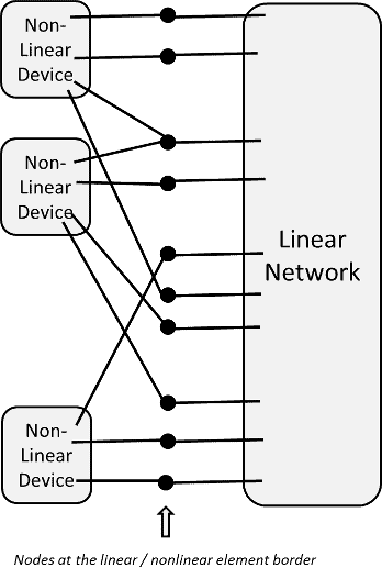
In Agile, non-linear devices can be embedded into subnetworks, and these are elaborated (expanded) into an overall structure as in the figure for the analysis. Although Agile allows harmonic balance simulation, it’s probably more used for linear analysis.

It provides the following features:

1. Advanced Network Descriptive Language (NDL). Allows network parameters to be defined in terms that relate algebraically.
2. Parametric, hierarchical circuit or system description. Sub-modeling allows users to create component models as any interconnection of AGILE circuit components or other sub-models.
3. AGILE is both a circuit and system level simulation and optimization tool.
4. True multi-port analysis allowing networks of any size to be analyzed in a convenient way.
5. Unlimited numbers of ports. frequencies. and all other attributes. AGILE allows circuits of any size or complexity to be analyzed up to system constraints.
6. Nonlinear circuit elements may be included at any sub-level in the circuit.
7. Output expressions allow network designers the ability to express the outputs as any algebraic combination of built-in output quantities.
8. Multi-port tabulated networks allow fixed data to be included in analyses.
9. Graphical output of AGILE as either rectangular or polar data plotting
10. Algebraically defined optimization goals allow users to very flexibly create network performance objectives for use with optimization in either or both time and frequency domains.
11. User may choose any of several optimizers.
12. Advanced time domain features allow users to apply time domain signals to one or many ports and inspect either time domain or frequency spectra at any port.
13. Statistical features include sensitivity and Monte-Carlo analysis.
14. Advanced noise-analysis features for linear circuits. including handling of multiports and a unique correlated noise current generator component.
15. Graphical user interface for both Windows and Linux.

Example

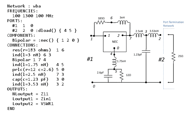
In the example here, a circuit named wba is defined in Agile, along with a depiction of the circuit. The example defines some frequency points, ports and components. A component named Bipolar uses a submodel called nec in the description; in this case nec is a linear model for a device, but it could be a nonlinear one as well. The output port (#2) uses a port termination network (dload which happens to be a load of 25 ohms), while the input port (#1) has the default system impedance load (50 ohms). Z-parameter and input impedance outputs are requested, along with VSWR at port 1. This example is very simple; of course, any of the many outputs could be used, and these can be combined using expressions to form new outputs.

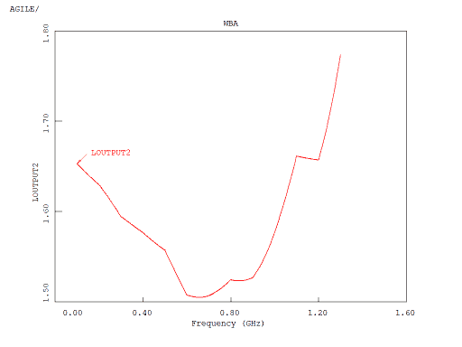Some   of the results from this circuit are shown here. We see the input impedance charted in polar form and the VSWR in rectangular form.

Here’s another example that shows more of Agile’s expressive capabilities.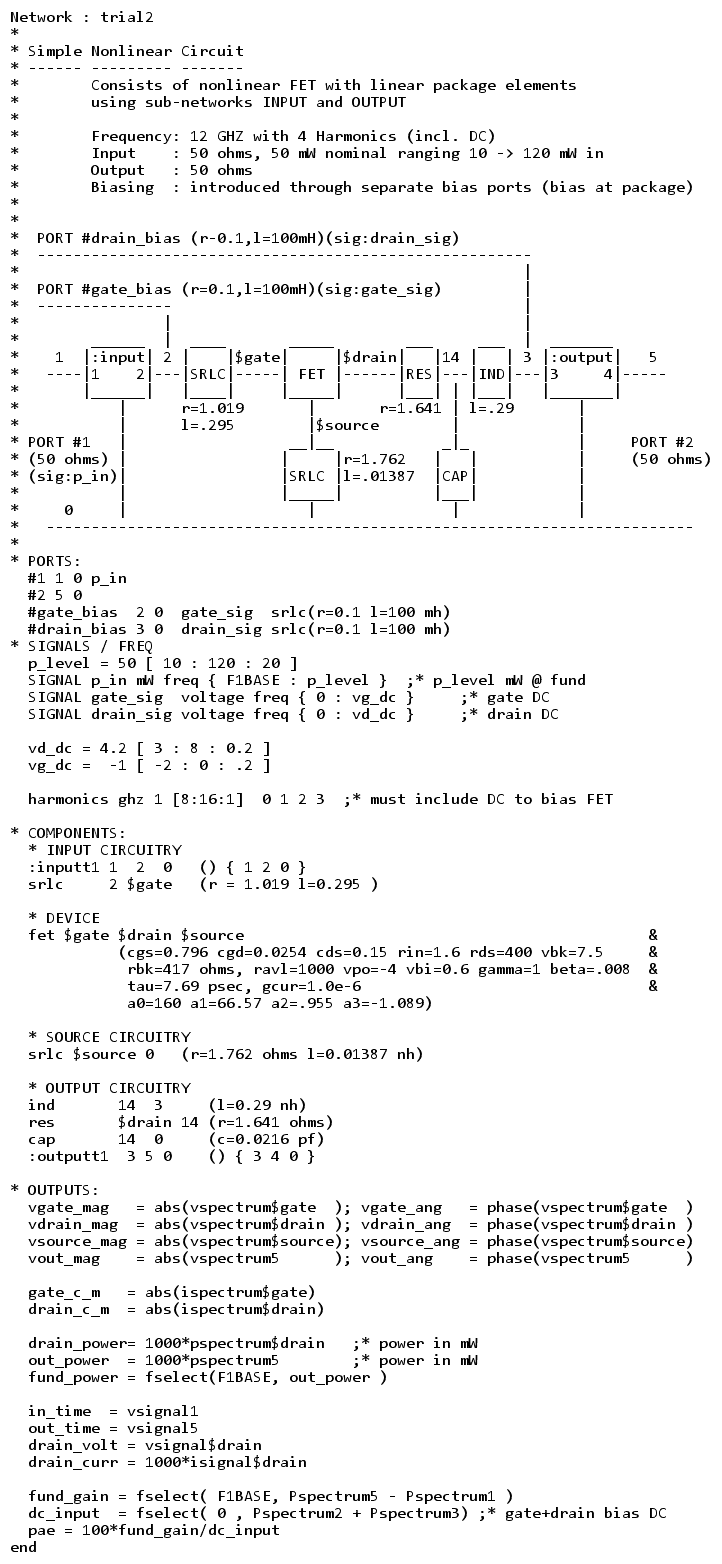

In this example, we see a non-linear FET model with biasing and input and output circuitry. A RF signal, p_in, is applied at the input and we examine various outputs and signals at various points in the circuit. We see a small sampling of use of expressions in Agile’s descriptions here.

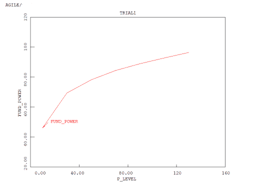
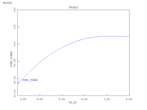
In the example outputs, we see the power in the fundamental versus input power; this shows compressive effects. Another graph shows the power in the fundamental versus drain bias (DC). And another graph shows the `op-cycle’ which is the voltage and current as they vary in time over an analysis cycle. This graph is for the sum of all harmonics (here we have the fundamental and the second and third harmonic), but you can also look at just a particular harmonic.

There’s lots more that you can do and more in the User Manual too, but here are some more quick examples. All of the graphs were generated using the tool.

Analysis

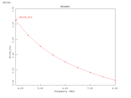
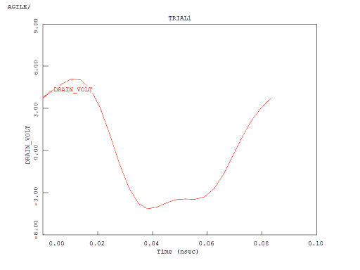
In one figure, we see the noise figure for a linear circuit across a frequency range. In the other one, we see the voltage at the drain of an FET amplifier in a non-linear circuit in the time domain. In this case, we see only one cycle of the output but there are settings to see multiple cycles if desired. Of course, since the analysis takes place in the frequency domain, each of these cycles is the same.

Optimization

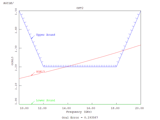
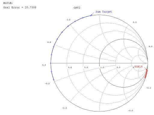
Optimization goals can be defined using upper and lower bounds. In that case shown here, the goal is not being met since it is not completely contained within the required bounds. Optimization goals can be defined in the complex domain as well as seen in the other graph. In this case, the goal error reflects the difference between the desired points and the actual points in the complex plane. The optimization goal, the figure of merit, can be very flexibly defined using the algebraic features of the program to combine goals like these as well as other expressions.

Statistical Analysis and Design

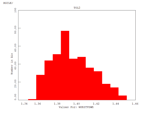
Sensitivity analysis, tolerance analysis (via Monte-Carlo methods) and tolerance design (optimization of tolerance analyses) are features of the program. Just as a generalized expression can be used to define a figure of merit for optimization purposes, a generalized expression can be used to define cost which is the target for tolerance design. In one figure, we see a ‘manual’ means of seeing the effect of changing a variable on a reflection coefficient result. In the other figure, we see the resultant VSWR histogram after a tolerance analysis run.